As a Board Member of the Microfluidics Association (MFA), I’ve gained several new insights about different areas of the microfluidics industry over the last few years, insights that are not apparent from my usual perspective as a product development consultant. One new area for me, and a major focus for the MFA, is that of product standards and standardisation; the MFA has had leading and supporting roles in the creation of three ISO microfluidics standards (ISO 22916:2022, ISO 10991:2023 and ISO/TS 6417:2025) over the last few years, with more in the funnel, some available as downloadable white papers on the MFA site.
A major thrust in this effort is the work from the earlier MFMET I project, and now as of June 2025, the newly funded MFMET II project, on whose advisory board I sit. The Portuguese members of this consortium (Instituto Português da Qualidade, NOVA School of Science and Technology, INESC MN and Instituto Superior Tecnico, Universidade de Lisboa), led by Elsa Batista (MFMET Project Coordinator and also Board Member for MFA) published an excellent paper in Frontiers in Nanotechnology last month entitled “Advancing calibration techniques for accurate micro and nanoflow measurements“. Their research compared 4 different flow rate calibration methods for microflow pumping (syringe pumps straight to calibration, and also pumping through a microfluidic chip first) and sensing, in terms of each method’s analytical performance as quantified by accuracy and precision (more on these terms later). This is really good, rigorous work which is important for the field of analytical chemistry, for other branches of chemistry, and for other sciences and fields of engineering.
The four calibration methods used were gravimetric (measuring the mass of a pumped volume of liquid), interferometric (measuring the linear displacement of the syringe plunger optically via laser interferometry), ‘front track’ (measuring the linear displacement of the leading meniscus of the water/air interface inside a capillary via high-resolution optical imaging) and ‘pending drop’ (measuring the size of a suspended, growing droplet via high-resolution optical imaging). These methods are shown schematically in Figures 1-4 from the paper, reproduced below as Figure 1.

As any trained scientist or engineer can imagine, arriving at a valid estimation of the different sources of error involved with any of these flow rate measurements is quite involved. For all methods, the volume pumped from the syringe was quantified gravimetrically by measuring the mass of water displaced over a given syringe plunger stroke distance. All measurement instrumentation had to be validated, so calibration certificates were obtained for analytical balances, chronometers and thermometers used. In some cases, established literature values for physical constants were used. Tables showing the different error components were included for each measurement approach, including factors such as temperature, expansion coefficients, evaporation, and buoyancy, in addition to direct measurements of mass, time and distance.
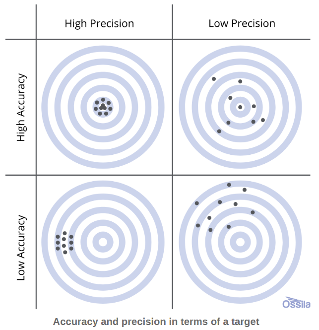
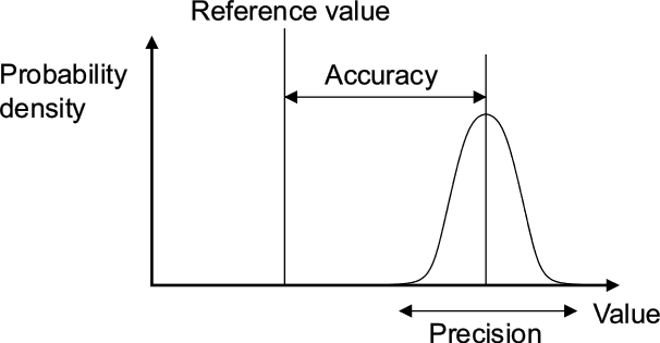
Since the methods are contrasted based on their accuracy and precision as quantitative measurements of error, it’s probably useful to define accuracy and precision as they are used scientifically: accuracy describes how close measurements are to a ‘target’ or reference value, while precision describes how close repeat measurements are to each other (regardless of accuracy). This is depicted well with a target practice analogy, as shown at right in Figure 2. In a scientific context such as the paper being highlighted, many replicate measurements are made of the variable in question (e.g. mass, volume, flow rate), to reduce the error measured by accuracy and precision. For most types of measurements (including those in this paper), if the measurements are binned and the number of measurements at any value are plotted against the value of the variable itself, a Gaussian distribution (or ‘bell’ curve) is produced. This is illustrated in Figure 3, below right. Here, the proximity of the centre of the bell curve to the ‘real’ value shows the accuracy of the measurements and method, while the spread of the measurements shown by the width of the bell curve shows their precision.
In addition (and unfortunately), sometimes different fields of science and/or geographic regions use different terms or units to describe the same thing (I think pressure is the poster child, here: atm, psi, kPa, hPa, bar, mbar, Torr, mm Hg … !!). In this paper, accuracy is analogously referred to as simply ‘error’, while precision is referred to as ‘uncertainty’. (Sidebar: these terms are poorly conceived, in my view, but my short foray into terminology standards leads me to believe that they arrive by royal decree from IUPAC (International Union of Pure and Applied Chemistry). All may not hail IUPAC, with (yet more) misses like this. Anyways, end of rant, back to the story!)
All four calibration methods were applied to a Nexus syringe pump operating at five flow rates ranging from 1-1000 µL/h, and the results shown in their Table 5, reproduced below as Figure 4. There’s a corresponding graph for this data, but unfortunately the data for each method were superimposed on each other at each flow rate, so the graph is hard to read. “Error (%)” is the relative accuracy, i.e. ((set point) – (measurement average)) / (measurement average) • 100%, while “U (%)”, uncertainty, is the relative standard deviation, RSD, or coefficient of variation, CV, of the measured values, i.e. RSD = CV = σ / (measurement average) • 100%, where σ is the standard deviation of the measured values.
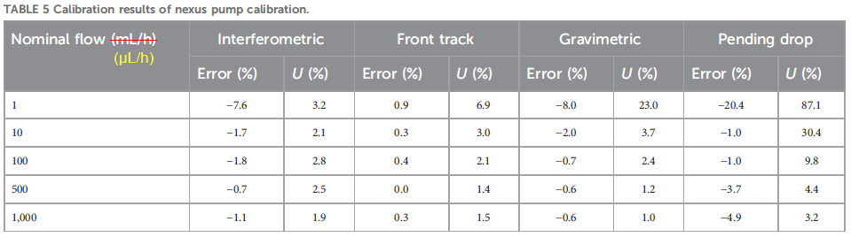
This table offers the best contrast of the methods, with the precision as RSDs (“U (%)”) telling the tale. The interferometric method is the clear winner, maintaining very respectable low single digit RSDs right down to the minimum 1 µL/h tested, while front track, gravimetric and pending drop could only do this at 10, 10 and 100 µL/h, respectively. Understandably, accuracy (“Error (%)”) goes down the drain once the RSDs skyrocket, indicating the method is no longer within its dynamic range.
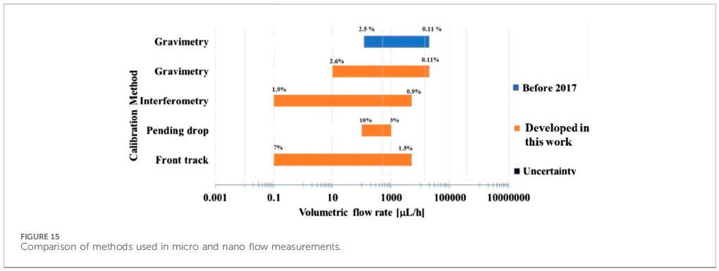
After looking at method performance for some other pumps, flow sensors, and with a chip coupled or decoupled, the team generated a bar chart in their Figure 15 to show the dynamic ranges for each method, including their previous gravimetric work. This figure is reproduced below as Figure 5.
The authors discuss the pros and cons of each method vis-à-vis their performance, highlighting that:
- the superior performance of the laser interferometric method is offset somewhat by the higher cost of instrumentation;
- the front track method is relatively inexpensive, and its precision (already good, IMO) could be improved with a smaller bore imaging capillary;
- the gravimetric method is inexpensive, simple to implement, and offers good performance; and
- the pending drop method could be improved significantly with better evaporation control.
Based on design and precision results, I would argue that the gravimetric method, while a step better than the pending drop method, is also more susceptible to evaporation, so improving evaporation control would likely improve both methods. There is also likely a way to make a diode laser-based interferometer that would be economical at volume, though I’m not sure that there are attractive applications that would warrant the product development.
This paper is solid and provides calibration information directly applicable to the pumps and flow sensors tested, but also and perhaps more importantly, information regarding the useful flow rate ranges for each calibration method. It’s a ‘nuts and bolts’ paper (like some I’ve written) that has no hope of reaching a flashy, high-impact journal, but which is of tremendous value, in my opinion, to microfluidic researchers and product developers in a variety of private sector, government and academic lab settings who can use this information as foundation material for their work.